Conditioning on robust summaries of the data in a Bayesian model is one way to achieve robustness to model miss-specification. I have called this the “restricted likelihood” here and here since the full data likelihood is replaced with the likelihood conditioned on only the robust summary (i.e. a restricted likelihood).
One of the easiest examples to conceptualize is outliers in a univariate setting. Suppose the true data generating mechanism is a contaminated normal:
\[y_1, y_2, \dots, y_n \sim (1-p)N(\mu, \sigma^2) + pN(\mu, c\sigma^2)\]
with \(c>1\) and we are interested in estimating \(\mu\). Since we don’t know the data generating mechanism exactly we just decide to fit the simple normal Bayesian model:
\[\mu \sim N(\eta, \tau^2),\]
\[\sigma^2\sim IG(\alpha, \beta),\]
\[y_1, y_2, \dots, y_n \sim N(\mu, \sigma^2)\]
Of course each data point gives information about \(\mu\) but the data coming from the contamination component gives less information about \(\mu\). Since we are fitting the wrong model it’s probably not good to treat these data points the same. In robust statistics, estimators like the median, trimmed-mean, or M-estimators down-weight outliers in a more or less automatic sense. In an analogous fashion, a Bayesian could condition on these robust summaries instead of the entire data set \(Y=(y_1, y_2, \dots, y_n)\). Though we have developed fitting methods to condition on such statistics (see above links to papers), for this post let’s condition on a middling set of order statistics \(T(Y)=(y_{(k)},y_{(k+1)},\dots, y_{(n-k)})\). The reasons being are 1) this is one of the first things I tried when starting to think about these problems and 2) the model is easy to fit since the pdf of a set of order statistics is analytically tractable (i.e. the restricted likelihood). This is not the case for many robust statistics like M-estimators).
The full posterior (conditioning on the full data) is \(\pi(\theta|Y)\propto \pi(\theta)f(Y|\theta)\) with \(\theta = (\mu, \sigma^2)\) while the “restricted posterior” is \(\pi(\theta|T(Y))\propto \pi(\theta)f(T(Y)|\theta)\) with \(f(T(Y)|\theta)\) just the pdf of the set of order-statistics. The function fitOrderStatistics in the (still developing) brlm package can be used to fit both of these models on a grid.
Demonstration
Let’s load the required packages and generate some data from the contaminated distribution:
library(reshape2)
library(tidyverse)
## Loading tidyverse: ggplot2
## Loading tidyverse: tibble
## Loading tidyverse: tidyr
## Loading tidyverse: readr
## Loading tidyverse: purrr
## Loading tidyverse: dplyr## Conflicts with tidy packages ----------------------------------------------## filter(): dplyr, stats
## lag(): dplyr, statslibrary(RColorBrewer)
#library(devtools); install_github("jrlewi/brlm") if needed. brlm=Bayesian Restricted Likelihood Methods.
library(brlm)
plotCors <- brewer.pal(9, 'Set1') #plot colors
#function to generated the contaminated data
gen_data <- function(n,mu, sigma, p, c){
out <- rbinom(n, 1, p)
sapply(out, function(ot) ifelse(ot, rnorm(1,mu, sqrt(c)*sigma), rnorm(1,mu, sigma)))
}
set.seed(8675309) #the Jenny seed :)
n <- 100
mu <-0
sigma <-1
p <- .2
c <- 10
y <- gen_data(n,mu, sigma, p, c)
ggplot(as_tibble(y), aes(x = value)) + geom_histogram(col = 1, fill = plotCors[2])## `stat_bin()` using `bins = 30`. Pick better value with `binwidth`.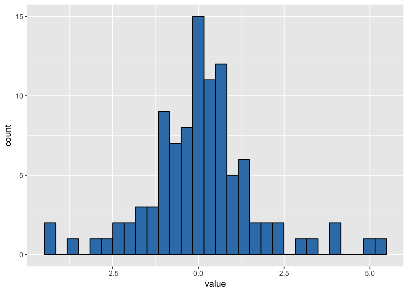
Now we can fit the models. The parameter k specifies the set of middling order statistics. Setting k=0 fits the full normal model.
mu_lims <- c(mu - sigma, mu + sigma) # play around with these since we are fitting on a grid. Just need to make sure grid covers support of non-zero posterior mass - MCMC would avoid this :)
length_mu <- 100
sigma2_lims <- c(.1, 5)
length_sigma2 <- 100

# fixed prior parameters
eta <- 2; tau <- 10; alpha <- 5; beta <- 5
k <- floor(.1*n)


fitFull <- fitOrderStat(y,k=0, mu_lims,length_mu, sigma2_lims,length_sigma2, eta, tau, alpha, beta)

fitRest <- fitOrderStat(y,k=k, mu_lims,length_mu, sigma2_lims,length_sigma2, eta, tau, alpha, beta)

post_mu <- tibble(mu = fitRest$muPost[,1], restricted = fitRest$muPost[, 2], full = fitFull$muPost[,2])
post_mu <- melt(post_mu, id.vars = c('mu'), variable.name = 'posterior')

post_sigma2 <- tibble(sigma2 = fitRest$sigma2Post[,1], restricted = fitRest$sigma2Post[, 2], full = fitFull$sigma2Post[,2])
post_sigma2 <- melt(post_sigma2 , id.vars = c('sigma2'), variable.name = 'posterior')


(p_post_mu <- ggplot(post_mu, aes(x = mu, y = value,  col = posterior)) + geom_line() +
  geom_vline(xintercept = mu, lty = 2) +
    xlim(c(mu - sigma, mu + sigma)))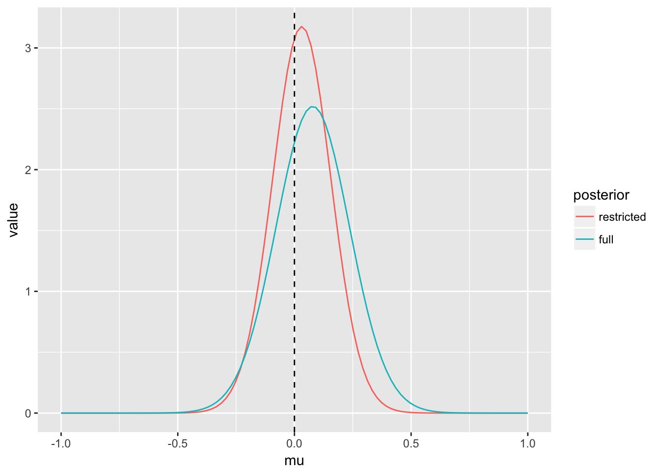
(p_post_sigma2 <- ggplot(post_sigma2, aes(x = sigma2, y = value,  col = posterior)) +
    geom_line() +
    geom_vline(xintercept = sigma^2, lty = 2) +
    xlim(c(0, 5)))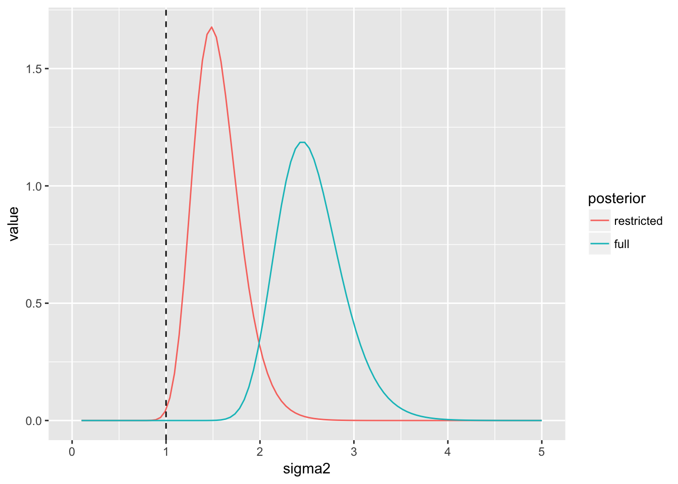
We see the posterior for \(\mu\) under the restricted posterior is more precise. This is related to the fact that estimation of \(\sigma^2\) is also improved under the restricted posterior.
Now suppose that the full model gets the likelihood correct - that is, the data are generated from a single normal:
set.seed(123)
y <- rnorm(n, mu, sigma)

fitFull_n <- fitOrderStat(y,k=0, mu_lims,length_mu, sigma2_lims,length_sigma2, eta, tau, alpha, beta)

fitRest_n <- fitOrderStat(y,k=k, mu_lims,length_mu, sigma2_lims,length_sigma2, eta, tau, alpha, beta)

post_mu_n <- tibble(mu = fitRest_n$muPost[,1], restricted = fitRest_n$muPost[, 2], full = fitFull_n$muPost[,2])
post_mu_n <- melt(post_mu_n, id.vars = c('mu'), variable.name = 'posterior')

post_sigma2_n <- tibble(sigma2 = fitRest_n$sigma2Post[,1], restricted = fitRest_n$sigma2Post[, 2], full = fitFull_n$sigma2Post[,2])
post_sigma2_n <- melt(post_sigma2_n , id.vars = c('sigma2'), variable.name = 'posterior')


(p_post_mu_n <- ggplot(post_mu_n, aes(x = mu, y = value,  col = posterior)) + geom_line() +
  geom_vline(xintercept = mu, lty = 2) +
    xlim(c(mu - sigma, mu + sigma)))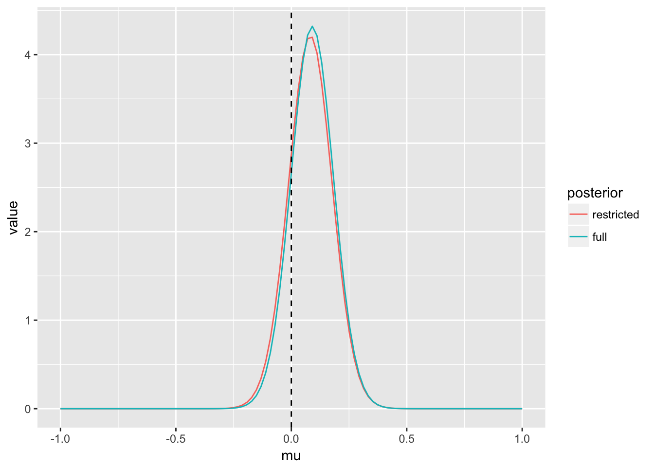
(p_post_sigma2_n <- ggplot(post_sigma2_n, aes(x = sigma2, y = value,  col = posterior)) +
    geom_line() +
    geom_vline(xintercept = sigma^2, lty = 2) +
    xlim(c(0, 5)))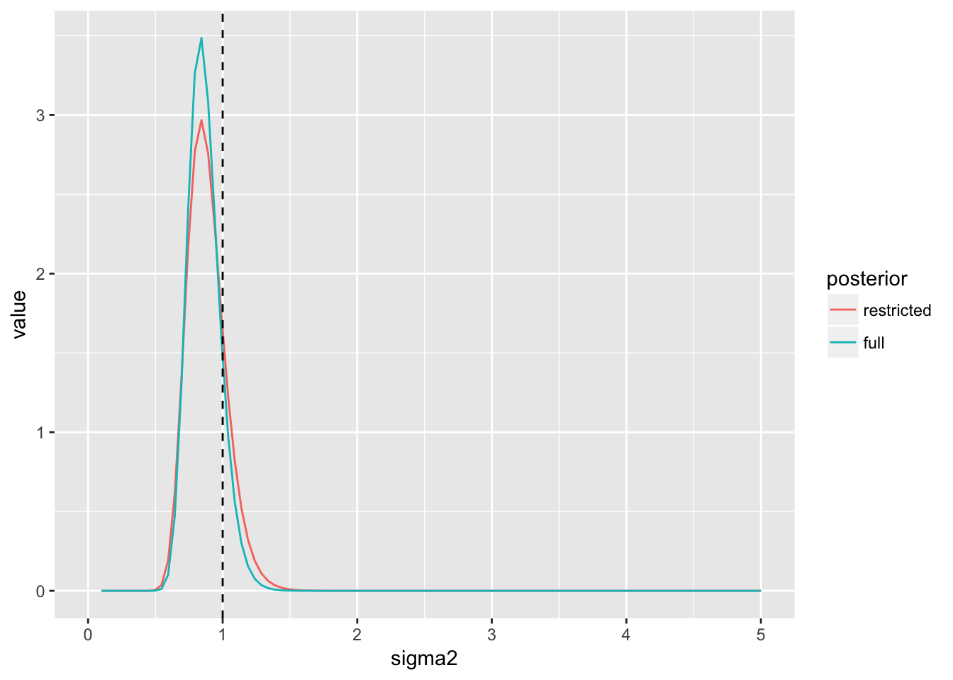
In this case - inference is essentially identical using either the restricted or full model - an often desired property of robust models.
Simulation
It’s probably best to re-do the analysis over several data sets. Here we generate 100 data sets from the contaminated model, fit the full and restricted posteriors, and summarize the posterior means. We’ll also try some parallelization using foreach.
library(doParallel)## Loading required package: foreach##
## Attaching package: 'foreach'## The following objects are masked from 'package:purrr':
##
## accumulate, when## Loading required package: iterators## Loading required package: parallelcl <- makeCluster(detectCores())
registerDoParallel(cl)
n_sims <- 100
(tm <- system.time({
result <- foreach(i = 1:n_sims, .combine = rbind, .packages = 'brlm') %dopar% {
y <- gen_data(n,mu, sigma, p, c)
fitFull <- fitOrderStat(y,k=0, mu_lims,length_mu, sigma2_lims,length_sigma2, eta, tau, alpha, beta)
fitRest <- fitOrderStat(y,k=k, mu_lims,length_mu, sigma2_lims,length_sigma2, eta, tau, alpha, beta)
c(fitFull$postMeans[1], fitRest$postMeans[1])
}
})[3])
registerDoSEQ()
result <- tibble(full = result[,1], restricted = result[,2])
result <- reshape2::melt(result, variable.name = 'posterior', value.name = 'mean mu')## No id variables; using all as measure variables(g_sim <- ggplot(result, aes(y = `mean mu`, x = posterior, fill = posterior)) + geom_boxplot())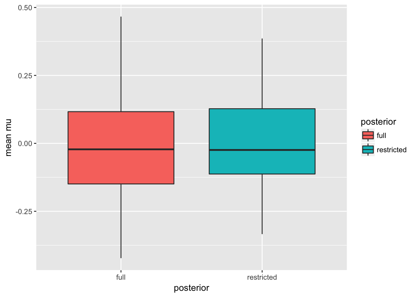
## elapsed
## 171.625
The means of the posterior means are roughly equal with smaller variance under the restricted posterior. The raw numbers are:
(sumry <- as.data.frame(result) %>% group_by(posterior) %>% dplyr::summarise(mean = mean(`mean mu`), sd=sd(`mean mu`)))## # A tibble: 2 x 3
## posterior mean sd
## <fctr> <dbl> <dbl>
## 1 full -0.005932405 0.1816344
## 2 restricted 0.002674353 0.1485771We see a reduction in standard deviation of roughly 18.2\(\%\) under the restricted posterior.
Summary
This was just a brief intro to the ideas and potential advantages of restricted likelihood methods. Conditioning on order statistics is conceptually simple and easy to implement since the pdf of order statistics is known. The choice of which order statistics to condition on is up for discussion. I have also developed MCMC methods to condition on M-estimators in regression settings (see this or this). Implementation in this settings is more difficult since the likelihood conditioned on such estimators is intractable. Code implementing some of these methods can be found here or here.